Rough Volatility as ML Benchmark

The two papers

Design Principle and Concrete Domain

Paper 1.8 — Cross-Domain Benchmark Principle

Rough volatility as a reusable benchmark design criterion

Both realized volatility forecasting (empirical, H ≈ 0.1) and semiconductor defectivity simulation (H = 0.1 by design) reward domain expertise at every pipeline layer. Partial corrections produce plausible-looking but still systematically wrong results — making shallow domain expertise detectable. The 7.1% instability loss in the fab simulation is visible only through path modeling; the static average erases it.

Four conditions. Two domains. One benchmark design principle.

Paper 1.9 — Concrete ML Evaluation Domain

Realized volatility forecasting as the financial benchmark

The generative process — fractional Brownian motion, H ≈ 0.1, validated across thousands of assets — is structurally incompatible with every standard ML architecture. LSTMs, Transformers, and AR models carry Markovian inductive biases that conflict with rough volatility. The mismatch is not tunable; it is architectural. HAR-RV is the expert floor, not the ceiling. An evaluator's job is to determine whether a practitioner knows to start there — and why.

Know the process before fitting any model. That is the bar.

What rough volatility is

H ≈ 0.1 — Rougher Than Brownian Motion

The Process

Fractional Brownian Motion

Realized volatility behaves like a fractional Brownian motion with Hurst exponent H ≈ 0.1 — empirically validated across thousands of assets by Gatheral, Jaisson, and Rosenbaum (2018). H < 0.5 means anti-persistent increments: positive moves are more likely to reverse than continue. At H = 0.1 the paths are substantially rougher than standard diffusions.

The Consequence

Clustering and Anti-Persistence Together

Volatility clusters at high levels — when it rains, it pours — while increments remain anti-persistent. This two-layer structure is what makes finite-context architectures structurally misspecified. Adding depth or attention heads does not fix a Markovian bias.

Four pipeline layers

Where The Naive ML Pipeline Fails

Layer 1

Feature Engineering

Default (wrong): raw daily returns. Domain-correct: log-realized variance at 5-minute, 1-hour, and daily frequencies plus bipower variation.

Raw daily returns have near-zero autocorrelation — the signal has already decayed. A model ingesting raw returns is fitting noise. This is not a hyperparameter problem; it requires knowing what the relevant process signal is.

Layer 2

Architecture Selection

Default (wrong): LSTM, Transformer, AR. Domain-correct: HAR-RV, rough fractional kernel, neural-SDE.

Standard architectures carry Markovian inductive biases that cannot represent fBm long-memory structure. The mismatch is architectural, not a scale problem. Deeper LSTMs do not resolve it.

Layer 3

Validation Protocol

Default (wrong): k-fold cross-validation. Domain-correct: expanding-window walk-forward with 252-day burn-in.

K-fold on a long-memory series allows future path information to contaminate training. In-sample metrics look strong; out-of-sample performance collapses during volatility regime shifts — exactly when the model is needed most.

Layer 4

Evaluation Metric

Default (wrong): MSE. Domain-correct: QLIKE.

MSE over-penalizes large absolute errors without normalizing by the current volatility level. QLIKE weights proportional errors and is the standard criterion for volatility model comparison (Patton, 2011). A model optimized on MSE is systematically miscalibrated during high-volatility regimes.

The interaction structure

Corrections Are Jointly Necessary

Three out of four is not enough

Wrong features mask architecture failure in-sample — the model overfits noise with sufficient capacity. Wrong validation masks both. Wrong loss hides miscalibration until an out-of-sample volatility spike. A practitioner who corrects any three but not the fourth still produces a systematically miscalibrated result.

Shallow knowledge is detectable

A practitioner who knows two of the four corrections will be confidently wrong in specific, diagnosable ways that a domain expert can predict before seeing the model output. This is what makes the domain high-signal benchmark territory: partial expertise produces confident wrong answers, not noisier correct ones.

The expert floor

HAR-RV Is Not A Simplification

Model

HAR-RV (Corsi, 2009)

A linear heterogeneous autoregression on daily, weekly, and monthly realized variance components. No hidden layers. No attention. Interpretable: each coefficient maps directly to the multi-scale persistence structure of the process. Hard to beat at standard evaluation horizons.

Why It Matters

It Is A Statement About The Process

HAR-RV encodes the heterogeneous structure of rough volatility directly. A practitioner who knows this domain knows to start here. A practitioner who does not will likely never produce HAR-RV through search — the standard ML instinct is to add complexity, not to remove it.

Empirical evidence — Paper 1.9

HAR-RV vs LSTM: Walk-Forward Results (S&P 500, 2001–2025)

Walk-forward validation on 6,264 out-of-sample predictions. Expanding window, 252-day burn-in. HAR-RV uses OLS on daily, weekly, and monthly realized variance components. LSTM trained on the same features with MSE loss — intentionally the wrong loss function, as the paper describes.

Full Period QLIKE Ratio

96.7×

LSTM / HAR-RV over 2001–2025. HAR-RV wins across all 6,264 predictions.

COVID 2020 QLIKE Ratio

265.9×

LSTM degrades worst precisely during the highest-stress period — when the model is needed most.

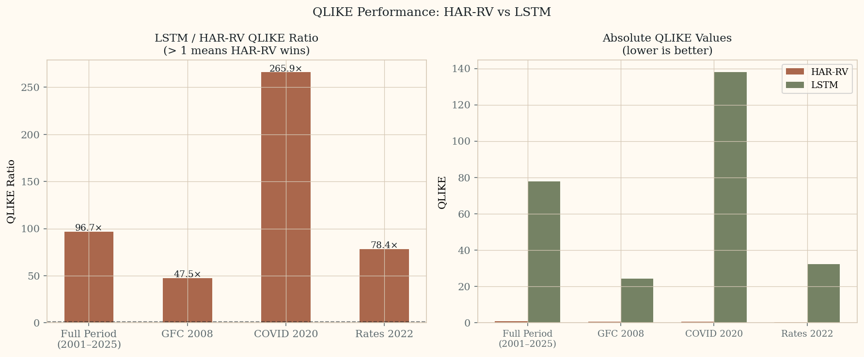
QLIKE ratio bar chart: LSTM vs HAR-RV by period

Left: LSTM/HAR-RV QLIKE ratio by period — values above 1 mean HAR-RV wins. Right: absolute QLIKE values — HAR-RV stays near zero across all periods while LSTM spikes at every stress event.

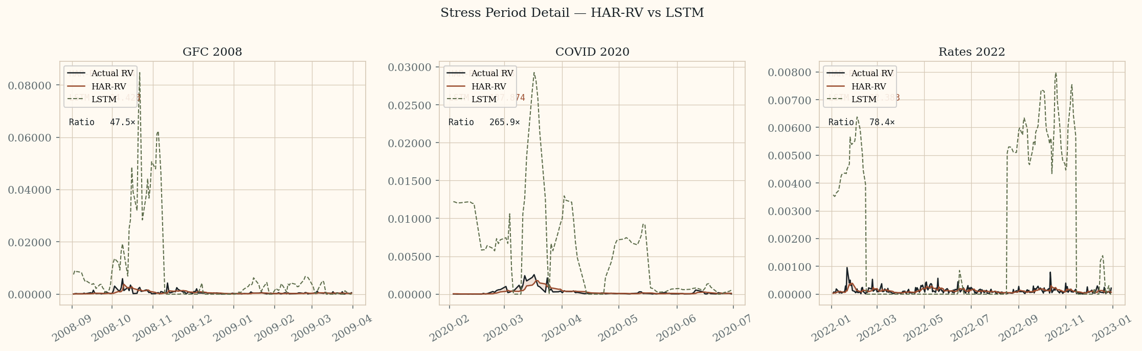
Stress period detail: GFC 2008, COVID 2020, Rates 2022

Stress period detail. HAR-RV (red) tracks actual RV (black) closely in all three periods. LSTM (green dashed) overshoots dramatically — particularly during COVID 2020 where it reaches 137.87 QLIKE vs HAR-RV's 0.518.

Cross-domain comparison

Two Domains, One Benchmark Property

Financial (empirical)

fBm, H ≈ 0.1, validated across thousands of assets. Default pipeline misses clustering through Markovian bias.

Semiconductor (modelled)

fBm, H = 0.1, design choice. Static D₀ average erases 7.1% instability loss visible only through path modeling.

Shared Failure

Naive pipeline produces plausible in-sample results that miss operationally significant behavior at regime shifts.

Shared Correction

Domain-informed structure owns the modeling correctness. The ML pipeline sits on top of it — it does not replace it.

Expert Bar

Know which pipeline choices are wrong for this process — and why — before fitting any model.

Four benchmark conditions

What Makes A Domain High-Signal For Testing Expertise

Condition 1

Structural Failures

Pipeline failures are correctable only by changing the modeling approach — not by tuning hyperparameters.

Condition 2

Process Knowledge Required

The correct approach at each layer requires understanding the process, not just fitting the data.

Condition 3

Pre-Fit Diagnosability

A domain expert can identify which pipeline choices are mismatched before fitting any model.

Condition 4

Partial Knowledge Is Detectable

Partial corrections produce plausible-looking but still systematically wrong results. Shallow domain expertise is visible.

One-line thesis

What These Papers Are Actually Saying

Domain expertise is testable. A practitioner who knows rough volatility can specify the correct pipeline before seeing the data — because they understand the process. One who does not will be confidently wrong in ways a domain expert can predict in advance.

Related work

Companion Site

The semiconductor simulation that motivated the cross-domain principle is documented at Fab Simulation & RVH — Paper 1.4.